Inductive Representation Learning on Large Graphs

(Hamilton et al., 2017)

Feb 03, 2026 Kisan Thapa GraphSAGE, Graph Learning, Inductive Learning

Abstract

GraphSAGE is a framework for inductive representation learning on large graphs. Unlike transductive methods (which require all nodes during training), GraphSAGE generates node embeddings for unseen nodes by learning a function that samples and aggregates features from a node's local neighborhood.

The Problem with Early GNNs (Like GCN)

Early GNNs were Transductive.

What that means: You have to feed entire graph into the training process.
The limitation: You have to retrain the whole model to generate an embedding if new node is added, or some property changed.
Scalability: You cannot easily process a graph with billions of nodes like (Pinterest or Facebook) because the whole adjacency matrix won't fit in GPU memory.

The GraphSAGE Solution

GraphSAGE (Graph Sample and Aggregate) introduced Inductive learning to graphs.

What that means: Instead of learning embeddings for each node, GraphSAGE learns aggregating Functions.
The Analogy:
- Transductive (GCN): Memorizing the map of New York City. If you go to London, you are lost.
- Inductive (GraphSAGE): Learning the skill of reading a map. You can now navigate New York, London, or a city that hasn't been built yet.
High-Level Intuition: assumes that a node is defined by its neighbors
1. Sampling: For a target node, select fixed number of neighbors (not all of them, just a sample). This keeps computation fixed regardless of node degree.
2. Aggregating: Gather the feature information (text, images, stats) from those sampled neighbors and squash them together into a single vector.
3. Updating: Combine the neighbors' aggregated info with the target node's current info to create a new embedding.

Method

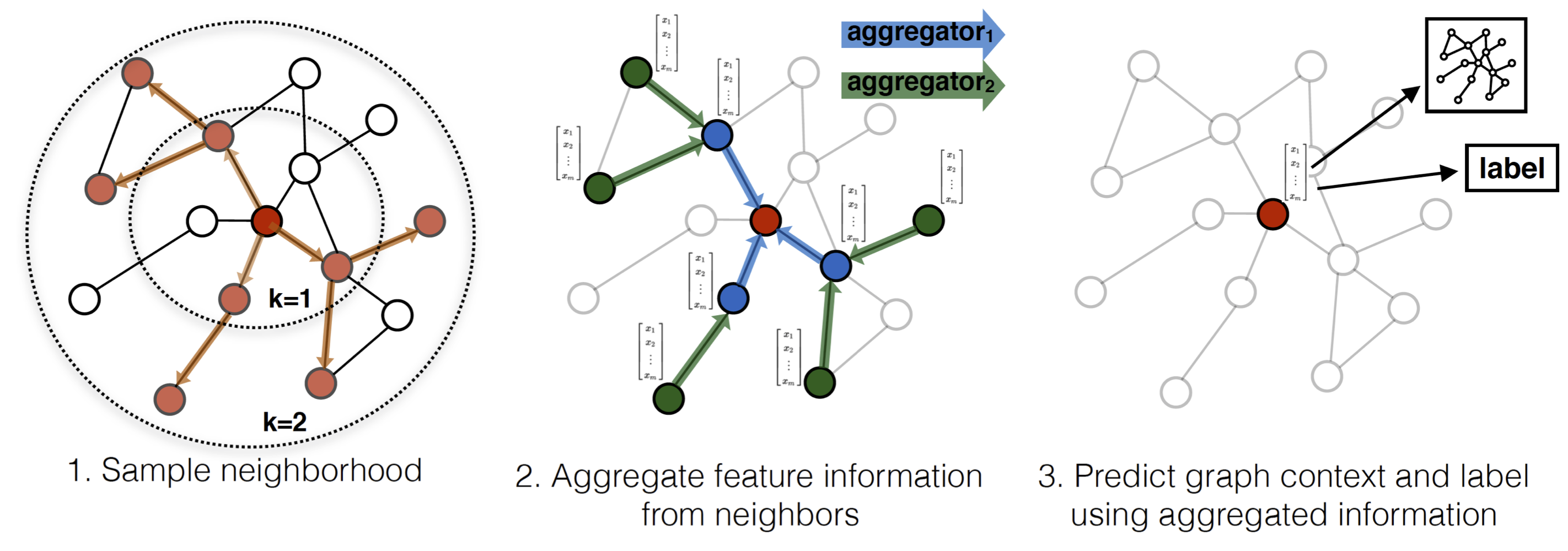
The GraphSAGE algorithm generates embeddings by aggregating information from a node's local neighborhood. The process consists of three main steps: (1) Neighborhood Sampling, (2) Aggregation, and (3) Prediction/Loss.

Forward Propagation Algorithm:
Let the graph be defined as $\mathcal{G} = (\mathcal{V}, \mathcal{E})$ with input features ${\{\mathbf{x}_v, \forall v \in \mathcal{V}\}}$. Let $K$ be the search depth (number of layers).
We initialize the vector representations at $k=0$ as the input features: \[ \mathbf{h}^0_v = \mathbf{x}_v \]

For each layer $k = 1 \dots K$, and for each node $v \in \mathcal{V}$:
1. Aggregate Neighbors: \[ \mathbf{h}^k_{\mathcal{N}(v)} = \text{AGGREGATE}_k \left( \{ \mathbf{h}^{k-1}_u, \forall u \in \mathcal{N}(v) \} \right) \]
2. Update Node Embedding:
  Combine the aggregated neighbor info with the node's own previous representation: \[ \mathbf{h}^k_v = \sigma \left( \mathbf{W}^k \cdot \text{CONCAT} \left( \mathbf{h}^{k-1}_v, \mathbf{h}^k_{\mathcal{N}(v)} \right) \right) \] where $\mathbf{W}^k$ is a learnable weight matrix and $\sigma$ is a non-linearity (e.g., ReLU).
3. Normalize: \[ \mathbf{h}^k_v = \frac{\mathbf{h}^k_v}{\| \mathbf{h}^k_v \|_2} \]
The final representation for node $v$ is $\mathbf{z}_v = \mathbf{h}^K_v$.
Aggregation Functions:
The aggregation function must be permutation invariant (the order of neighbors should not matter). The paper proposes three distinct architecture choices:
- Mean Aggregator:
  This is the simplest approach. It takes the element-wise mean of the vectors in $\{ \mathbf{h}^{k-1}_u, \forall u \in \mathcal{N}(v) \}$. \[ \text{AGGREGATE}_k^{\text{mean}} = \frac{1}{|\mathcal{N}(v)|} \sum_{u \in \mathcal{N}(v)} \mathbf{h}^{k-1}_u \] Note: The paper notes that a variant of this (GCN-like) can concatenate the node $v$ with its neighbors before averaging, but the inductive Algorithm 1 keeps them separate during aggregation.
- LSTM Aggregator:
  LSTMs have higher expressive capability but are not naturally permutation invariant. To fix this, GraphSAGE adapts LSTMs to sets by applying them to a random permutation of the neighbors. \[ \text{AGGREGATE}_k^{\text{LSTM}} = \text{LSTM} \left( [ \mathbf{h}^{k-1}_{u_{\pi(1)}}, \dots, \mathbf{h}^{k-1}_{u_{\pi(|\mathcal{N}(v)|)}} ] \right) \] where $\pi$ is a random permutation function.
- Pooling Aggregator:
  This explicitly models the permutation invariance. Each neighbor's vector is passed through a fully connected neural network, followed by an element-wise max-pooling operation. \[ \text{AGGREGATE}_k^{\text{pool}} = \max \left( \{ \sigma \left( \mathbf{W}_{\text{pool}} \mathbf{h}^{k-1}_u + \mathbf{b} \right), \forall u \in \mathcal{N}(v) \} \right) \] where max denotes the element-wise maximum operator. This captures distinct features from the neighborhood (e.g., "is there any neighbor that is a fraudster?").
Neighborhood Sampling (Minibatching):
To keep the computational footprint manageable, GraphSAGE does not use the full set $\mathcal{N}(v)$. Instead, it uniformly samples a fixed size set of neighbors.
Let $S_k$ be the sample size at layer $k$. If $|\mathcal{N}(v)| < S_k$, we sample with replacement; otherwise, we sample without replacement. This ensures the memory footprint per batch is fixed and predictable, regardless of the node degree.
Loss Function:
GraphSAGE can be trained in a supervised or unsupervised manner.
- Unsupervised (Negative Sampling):
  We want nearby nodes to have similar embeddings, and disparate nodes to have distinct embeddings. For a node $u$, the loss function is: \[ J_{\mathcal{G}}(\mathbf{z}_u) = - \log \left( \sigma(\mathbf{z}_u^\top \mathbf{z}_v) \right) - Q \cdot \mathbb{E}_{v_n \sim P_n(v)} \left[ \log \left( \sigma(-\mathbf{z}_u^\top \mathbf{z}_{v_n}) \right) \right] \] where $v$ is a neighbor (positive sample), $P_n$ is a negative sampling distribution, and $Q$ is the number of negative samples.
- Supervised:
  For tasks like node classification, the unsupervised loss is replaced by a standard Cross-Entropy loss calculated on the final embeddings $\mathbf{z}_v$ of labeled nodes.

Python


  import sys
  import torch
  import torch.nn.functional as F 
  from torch_geometric.nn import SAGEConv
  from torch_geometric.datasets import Planetoid

  print(sys.version)
  print(torch.__version__)
  # 3.12.2 | packaged by conda-forge | (main, Feb 16 2024, 20:54:21) [Clang 16.0.6 ]
  # 2.10.0

  # Load cora citation data
  dataset = Planetoid(root="/tmp/Cora", name="Cora")
  data = dataset[0]
  print(type(data))
  # 

  # Graph Global Statistics
  print(f"Nodes: {data.num_nodes}")
  print(f"Edges: {data.num_edges}")
  print(f"Average node degree: {data.num_edges / data.num_nodes:.2f}")
  print(f"Isolated nodes: {data.has_isolated_nodes()}")
  print(f"Self-loops: {data.has_self_loops()}")
  print(f"Is undirected: {data.is_undirected()}")

  # Feature and Label Analysis
  print(f"Number of features: {dataset.num_features}")
  print(f"Number of classes: {dataset.num_classes}")

  # Class Distribution in Training Set
  train_labels = data.y[data.train_mask]
  values, counts = torch.unique(train_labels, return_counts=True)
  for v, c in zip(values, counts):
      print(f"Class {v.item()}: {c.item()} training samples")

  # Connectivity Inspection
  edge_index = data.edge_index
  print(f"Edge Index Shape: {edge_index.shape}")
  # Display first 5 edges
  print(edge_index[:, :5])

  """
  Output Context:
  Nodes: 2708
  Edges: 10556
  Average node degree: 3.90
  Isolated nodes: False
  Self-loops: False
  Is undirected: True
  Number of features: 1433
  Number of classes: 7
  Class 0: 20 training samples
  Class 1: 20 training samples
  Class 2: 20 training samples
  Class 3: 20 training samples
  Class 4: 20 training samples
  Class 5: 20 training samples
  Class 6: 20 training samples
  Edge Index Shape: torch.Size([2, 10556])
  tensor([[ 633, 1862, 2582,    2,  652],
          [   0,    0,    0,    1,    1]])
  """

  # Define GraphSAGE Model
  class GraphSAGE(torch.nn.Module):
      def __init__(self, in_channels, hidden_channels, out_channels):
          super().__init__()
          
          # Layer 1: Aggregates information from 1-hop neighbors
          self.conv1 = SAGEConv(in_channels, hidden_channels, aggr='mean')
          
          # Layer 2: Aggregates information from 2-hop neighbors (neighbors of neighbors)
          self.conv2 = SAGEConv(hidden_channels, out_channels, aggr='mean') 
          
      def forward(self, x, edge_index):
          # Step 1: Convolve (Aggregate neighbor info)
          x = self.conv1(x, edge_index)
          
          # Step 2: Activation (Add non-linearity)
          x = x.relu()
          
          # Step 3: Regularization (Prevent overfitting)
          x = F.dropout(x, p=0.5, training=self.training)

          # Step 4: Second Convolution
          x = self.conv2(x, edge_index)
          
          return F.log_softmax(x, dim=1)
      
  # Initialize
  device = torch.device('cuda' if torch.cuda.is_available() else 'cpu')
  model = GraphSAGE(dataset.num_features, 64, dataset.num_classes).to(device)
  data = data.to(device)
  optimizer = torch.optim.Adam(model.parameters(), lr=0.01, weight_decay=5e-4)

  # Training loop
  def train():
      # 1. Prepare the model
      model.train() 

      # 2. Reset Gradients
      optimizer.zero_grad()
      
      # 3. Forward Pass (The Prediction)
      out = model(data.x, data.edge_index)

      # 4. Calculate Loss (The Error)
      loss = F.nll_loss(out[data.train_mask], data.y[data.train_mask])
      
      # 5. Backward Pass (The Learning)
      loss.backward() 
      optimizer.step()
      
      return loss.item()

  # Run it
  for epoch in range(22):
      loss = train()
      print(f'Epoch {epoch}: Loss {loss:.4f}')

  """
  Epoch 0: Loss 1.9501
  Epoch 1: Loss 1.6858
  Epoch 2: Loss 1.2758
  Epoch 3: Loss 0.8277
  Epoch 4: Loss 0.4822
  Epoch 5: Loss 0.2450
  Epoch 6: Loss 0.1192
  Epoch 7: Loss 0.0669
  Epoch 8: Loss 0.0340
  Epoch 9: Loss 0.0196
  Epoch 10: Loss 0.0093
  Epoch 11: Loss 0.0098
  Epoch 12: Loss 0.0036
  Epoch 13: Loss 0.0028
  Epoch 14: Loss 0.0012
  Epoch 15: Loss 0.0023
  Epoch 16: Loss 0.0013
  Epoch 17: Loss 0.0012
  Epoch 18: Loss 0.0005
  Epoch 19: Loss 0.0023
  Epoch 20: Loss 0.0011
  Epoch 21: Loss 0.0004
  """

References

Hamilton, W. L., Ying, Z., & Leskovec, J. (2017). Inductive Representation Learning on Large Graphs. Advances in Neural Information Processing Systems (NeurIPS), 30.
Kipf, T. N., & Welling, M. (2017). Semi-Supervised Classification with Graph Convolutional Networks. International Conference on Learning Representations (ICLR).